Written by Jelle Mes
Abstract
In 2024 a large increase in young mussels (Mytilus edulis) was observed in the Dutch Wadden Sea. Mapping these reefs is time-consuming and cannot be done on a regular basis. Therefore we adapt a remote-sensing based approach to automate this process, which enables monthy observations. We also give a detailed background on the utilized synthetic aperture radar (SAR) techniques. This method is subsequently used to map reefs around the supratidal shoal Engelsmanplaat – we find a 25 fold increase in reef area in 2024 (see animation) This method can be readily applied to larger parts of the Wadden Sea, allowing for frequent & reliable measurements on the distribution and size of mussel reefs.
Mussel and their reefs
Mussels (specifically the species Mytilus edulis) form an important part of the ecosystem of the Wadden Sea. They filter the sea water for nutrients and excrete the remnants in the form of a fine, sticky mud that piles up and forms high reefs that stick out above the surroundings . They attach themselves mainly to hard surfaces such as rocks, buoys, shells and other mussels, forming dense three dimensional structures. This in turn forms the basis for other organisms to attach to, forming entirely new ecosystems. The mussels themselves are also an important food source for the Eurasian oystercatcher (Haematopus ostralegus; which actually does not feed on Japanese oysters, see below) and the Common eider (Anas mollissima) .
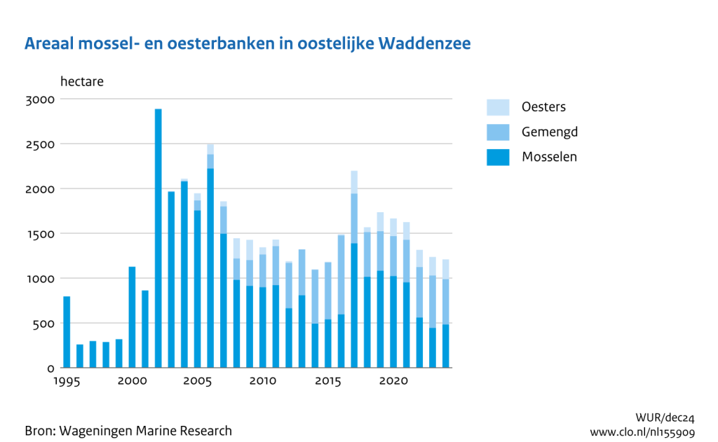
In the Wadden Sea the mussel reefs are located in both littoral (intertidal, on the mudflats) and sublittoral (permanently submerged) zones. Here we will focus on the intertidal zone, as this is more readily probed using remote sensing techniques. Since 2002 there has been a growing number of reefs of Japanese oysters (Crassostrea gigas), which often form mixed reefs with mussels . Of the 1236 hectares of intertidal reefs in the eastern Dutch Wadden Sea, 585 (47.3%) were mixed and 207 (16.7%) were oyster-only . In this work we do not make this distinction and refer to all as “mussel reefs”. By far most new reefs in 2024 are pure mussel reefs.
The current method of measuring the size of mussel reefs is by walking around each of them with a GPS device in hand during low tide, using the resulting GPS track as the basis for a polygon measuring the area . For the Dutch Wadden Sea this work is performed yearly by Wageningen Marine Research (WMR, formerly known as IMARES).
This is very labour intensive and cannot be done frequently. Instead, we propose using satellite imagery to measure these reefs directly. This is inexpensive as the remote sensing data is already openly available through the Copernicus Browser of the European Space Agency (ESA). The frequency of available imagery depends on the satellite platform, with radar having a higher effective revisit time than optical due to the effects of clouds. The downside to this remote sensing method for detecting the reefs is that we currently cannot make a distinction between oyster and mussels based on this data alone.
Growth in 2024 & in-situ observations
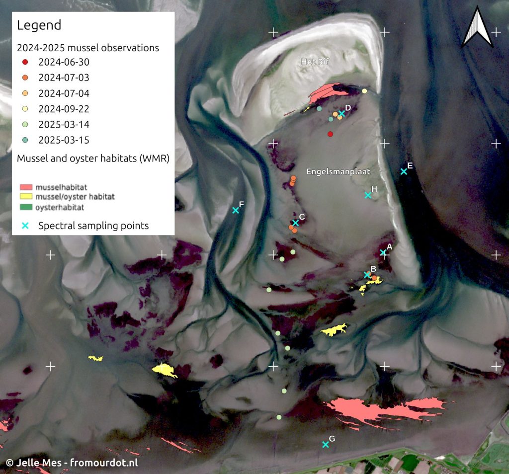
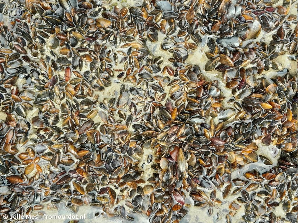
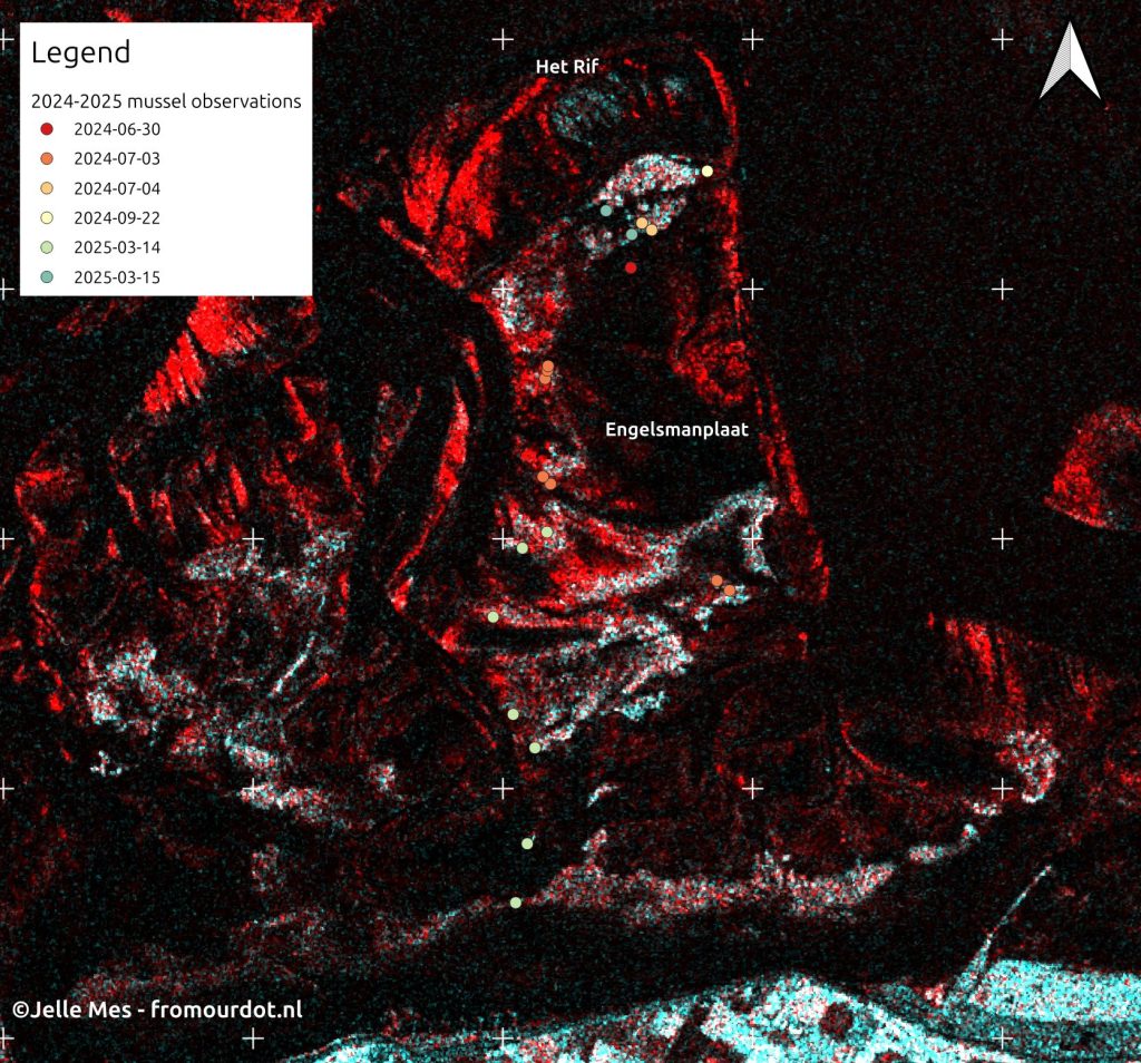
In 2024 a large increase in mussel population was observed throughout the Dutch Wadden Sea . One specific region where this occurred is the Engelsmanplaat, a supratidal shoal between the islands of Ameland and Schiermonnikoog, located in the Frisian Inlet. Volunteers of Staatsbosbeheer saw young (~5 mm) mussels spread over large areas near the tidal channels at the edge of the shoal. Fig. 2 shows the spread of mussel observations around the Engelsmanplaat compared to the up to then known location of mussel reefs (which in 2023 covered an area of roughly 11 hectares).
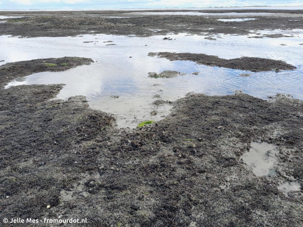
The young mussels did not stick out much above the intertidal seafloor in most places (e.g. Fig. 3) though in some spots near older mussel reefs more 3D structure was starting to appear (Fig. 4). This matches the development of reefs as described above.
Mussel reefs in optical satellite imagery
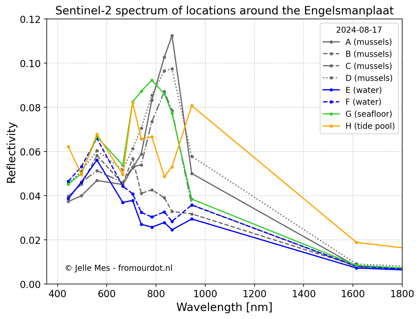
Observations were mostly made at the edge of the fields of young mussels, in part to avoid disturbing their natural development. The reefs can be recognized in Fig. 2 as dark patches outside of the tidal channels, with the observations located mostly at the edge of those patches. Selecting areas of mussels cannot be done based on this RGB image alone. In fact, even having the entire spectrum covered by Sentinel-2 will not always suffice. Fig. 5 demonstrates this with spectra from several locations of known new fields of mussels and other locations around the Engelsmanplaat not covered by mussels. Most of the locations (A, C and D) with mussels have relatively high reflectivity in the red edge and NIR bands (B07, B08, B8A), though location B has a surprisingly low reflectivity in these bands and is quite similar in spectrum to the two locations in water covered tidal channels (E and F). A, C and D have spectra similar to location G, which is an exposed intertidal seafloor with a relatively high abundance of surface covering algae, making those difficult to distinguish. This is because mussel shells are often covered in algae, therefore giving off similar spectral signatures as algae covered sediments and vegetation .
Aside from the difficulty in distinguishing features in the intertidal zone, the other large drawback of optical imagery is the impact clouds have on the availability of imagery. The Netherlands is notorious for the many cloudy days it has each year, with 2024 having only 14 instances of cloud-free imagery in the region of interest (the Frisian Inlet). Two additional complicating factors are the tide and the turbidity of the water. Mussel reefs cannot be exposed above the water for more than ~2 hours per tidal cycle . At the Engelsmanplaat, with water levels at the nearest tidal gauge in the range of -1.5 to +1.25 m NAP (local ordinance datum), mussel reefs do not form above roughly +0.1 m NAP. Most of the time the water in the Wadden Sea is non transparent due to the high turbidity, so imagery during high tide generally cannot be used to map the mussel reefs. This leaves only at most 2 h/12 h = 17% of the non-cloudy images available for use. In 2024 these low tide Sentinel-2 images are on the following 3 dates:
- 2024-07-30
- 2024-08-17
- 2024-10-26
The following dates have Sentinel-2 images of the Engelsmanplaat where lower water turbidity allows partial visibility of mussel reefs:
- 2024-05-21
- 2024-06-25
- 2024-07-15
- 2024-07-20
- 2024-09-21
Overall, optical satellite imagery would allow for mapping the mussel reefs primarily in the summer months, thus giving a roughly yearly overview . Another remote sensing method allows us to map the mussel reefs much more frequently: radar.
Mussel reefs in synthetic aperture radar (SAR) satellite imagery
Synthetic Aperture Radar (SAR) maps the Earth’s surface by sending radar signals sideways at the Earth and measuring the return signal. By combining return signals from the same point on the Earth which were received at different points along the orbital track of the satellite, one can achieve a much higher resolution than possible for a static radar system: the so called “synthetic” aperture versus the much smaller physical aperture of the radar system itself. Radio waves can easily penetrate the atmosphere at all atmospheric conditions and do not rely on the Sun illuminating the surface. Therefore images can be taken at any time of day regardless of the weather. This makes it possible to do frequent monitoring of the Earth’s surface with a regular cadence, unlike optical satellite imagery.
There are three quantities that can be measured with respect to the original emitted radar signal:
- Backscatter intensity \gamma_0 : the ratio of emitted versus received signal strength, corrected for the incidence angle on the Earth’s surface using a digital elevation map (DEM).
- The change in polarization: when a vertical (V) polarized radio wave is sent out, it returns partially in both vertical (V) and horizontal (H) polarization, so called co- (VV) and cross-polarization (VH). In a similar way, when a H polarized signal is emitted, it can return H and V, abbreviated as HH and HV.
- The phase difference between the emitted and received signals, used for instance in interferometric SAR (InSAR), which can measure surface elevation changes.
The backscatter intensity and polarization are important components for our investigation into mussel reefs. Therefore I will discuss these more in detail. The phase difference is less useful as the signal to noise ratio (SNR) is generally to low to extract this reliably.
Backscatter intensity
In the interaction between the emitted radar signal and the Earth’s surface there are three main categories :
- Double bounce: high \gamma_0
- Volumetric scattering: intermediate \gamma_0
- Surface scattering: low to intermediate \gamma_0 , depending on the roughness of the surface
The double bounce is an effect where a beam incident on two surfaces which are perpendicular to each other, like the wall of a building on flat ground, results in a direct return of the signal. This is similar to the effect of a corner radar reflector which can be found on buoys. Volumetric scattering on the other hand occurs in the tops of trees and other dense vegetation, occurring in a volume instead of at a surface interaction layer. The depth of penetration depends on the wavelength: longer wavelengths/lower frequencies penetrate deeper into a tree canopy. Lower in a tree canopy there are more vertically oriented objects (tree trunks) and these reflect the vertically polarized component of the radar pulse stronger than the horizontal component (see also below about polarization).
The third category, surface scattering, has a large dependence on the roughness of the surface quantified by the (mean) size of surface variations d . On the perfectly smooth end of this range the surface acts as a mirror, reflecting 100% of the radar pulse energy away from the source (the signal is always emitted sideways to the Earth’s surface, not nadir/top down): d < d_{smooth} . On the other side of this range is a surface with such a degree of roughness that an incoming radar wave is scattered in all directions with equal intensity. Such a surface is called “saturated” :, with d > d_{rough} . In between these extremes is a regime in which diffuse scatter increases and specular reflection decreases with increasing surface roughness: d_{smooth} < d < d_{rough} . The two transitions in roughness are given by the following equations, depending on radar wavelength \lambda and incidence (off-nadir) angle \theta_i :
- Radar smooth: d_{smooth} = \frac{\lambda}{25 \cos(\theta_i)}
- Radar rough: d_{rough} = \frac{\lambda}{4.4 \cos(\theta_i)}
The SAR platform that we will be using is Sentinel-1, with an operating C-band frequency of 5.405 GHz, equivalent to 5.55 cm wavelength. It’s off-nadir angle ranges from 29.1^{\circ} - 46.0^{\circ} . At an intermediate angle of \theta_i = 40^{\circ} , the two transition sizes are:
- d_{smooth} = 2.9\,\text{mm}
- d_{rough} = 16.5\,\text{mm}
The table below indicates roughness d for various surface types in the Wadden Sea with associated backscatter intensity measurements in the two polarization channels of Sentinel-1 (more on this in the next section). Due to the roughness of a mussel bed, one can expect a high radar backscatter there. Sand particle sizes are much smaller than d_{smooth} , so a flat surface of sand acts as a mirror to C-band radar, as shown for instance on the Engelsmanplaat (ignoring the effects of burrows of Arenicola maritima . The same is true for mud. However, sand, as a larger grained material, exhibits larger surface ripples when exposed to waves or strong currents. These result in a high backscatter, for instance at the Rif – west site. In general for bare intertidal flats, backscatter is dominated by surface ripples .
| Surface type | Location | d [mm] | C-band scattering type | VV \gamma_0 | VH \gamma_0 | Source for d |
|---|---|---|---|---|---|---|
| Sea water – surf zone | North Sea shorefront | ~ 5 | Rough – intermediate | 0.1 | 0 | |
| Sea water – no wave breaking | Tidal basin | < 1 | Specular | 0.01 | 0 | |
| Sand – smooth | Engelsmanplaat | 0.18 | Specular | 0.01 | 0 | SIBES |
| Sand – wave pattern | Rif – west | ~ 20 | Rough – saturated | 0.6-3 | 0 | |
| Mud | Wierummerwad – near shore | 0.04 | Specular | 0.01 | 0 | SIBES |
| Mussels – 1st year spring | Wierummerwad | ~ 15 | Rough – intermediate | 0.04-0.1 | 0 | |
| Mussels – 1st year autumn | Wierummerwad | ~ 35 | Rough – saturated | 0.1-0.7 | 0.02-0.1 |
Table 1: overview of various surface types and corresponding scattering modes and polarization signals. Polarization signals are measured in a Sentinel-1 image of 2024-12-17 of the Engelsmanplaat.
Polarization
As noted before, a radar signal is a mix of four flavours: VV, VH, HH, HV (see also the polarization matrix below). The components on the diagonal, VV and HH, are called co-polarized, while those off-diagonal, VH and HV, are called cross-polarized. The strength of these components depends on the shape of the surface/object that the radar signal interacts with, as demonstrated in Fig. 6. For instance, tree trunks, which are mainly oriented vertically, reflect mainly the vertically polarized wave strongly, and vice versa. Objects (or parts thereof) that do not have a preferred orientation (e.g. round leaves) or are distributed in random orientations, return both V and H polarization in equal strength.
| Send | |||
| V | H | ||
| Receive | V | VV | HV |
| H | VH | HH | |
Table 2: the four radar polarization modes.
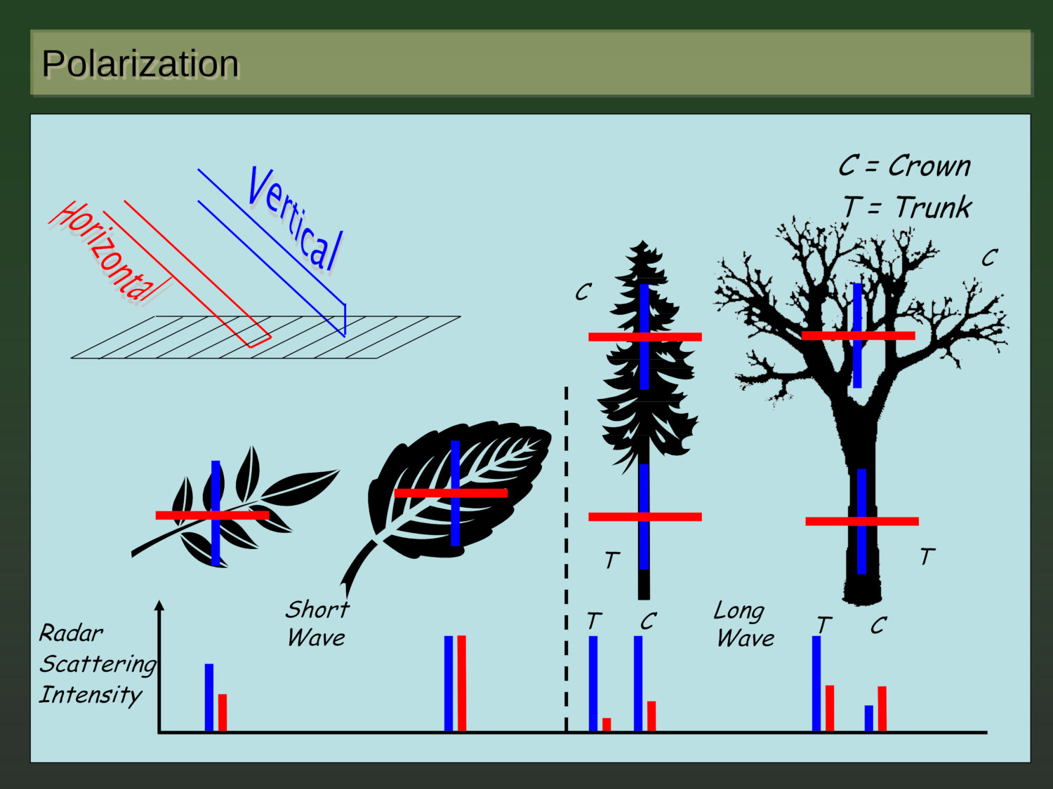
A good way to look at this is to imagine your object as a conductive (metal) rod: the oscillating electric field of the radar beam makes electrons in the rod oscillate too. This oscillation is easier in the long axis of the rod. The movement of the electrons in turn creates an oscillation in the electric field, which manifests itself as a radio signal traveling back towards the radar source. A field of vertical rods will therefore scatter/reflect the vertical V component strongly and allow any horizontal H to pass through.
So far we have only discussed the reflection of the V and H polarizations, the VV and HH components, which are on the diagonal of the polarization matrix (Table 2). The off-diagonal components, VH and HV, are made when the objects are not perfectly horizontal or vertical. For instance, if we have our conductive rod diagonally at 45 degrees, then a V signal can still make the electrons move along the length of the rod, albeit a “bit” less. The generated electromagnetic wave has a diagonal orientation, which is picked up on by both the horizontal and vertical antennae on our radar instrument. Therefore, we have equal parts VV as VH strength (ignoring orientation effects). This effect is known as “depolarization”, as a originally polarized siganl (V or H) is converted in a mix of polarizations, therefore getting less polarized.
Now finally imagine a field of randomly oriented rods and we send a V pulse to it. Some rods are oriented vertically and return the signal perfectly, others are oriented horizontally and return no signal at all, while most are somewhere in between these two orientation extremas and return a “bit” of V and H. Thus we get intermediate signal strength in both VV and VH modes. Instead of randomly oriented rods we have randomly oriented mussels: these have the same effect on the final polarization measurement.
Now comes Sentinel-1: in the Interferometric Wide Swath (IW) mode at 5 x 20 m resolution, which is the default observation scenario in Europe, the polarization mode is VV-VH . HH-HV is used for monitoring ice and snow in the polar regions. Therefore, we should be able to detect mussels as having a high VH to VV ratio in the Sentinel-1 images. Indeed, for large enough mussels, we see a significant VH component. All other surface types do not yield any VH signal. This effect was also observed by who also used SAR imagery to observe bivalve beds in the Wadden Sea.
Existing methods for mussel reef detection
In the past several papers have been published where the authors try to detect bivalve (mussel & oyster) reefs using SAR. utilize L, C and X-band radar to characterize elements on the intertidal seafloor. They use the spatial and temporal mean and standard deviation of co-polarization channels VV and HH or TerraSAR-X to detect mussel reefs in the German Wadden Sea. However, they cannot reliably distinguish between mussel reefs and other causes of surface roughness such as burrows of sand worms (Arenicola marina). also utilize TerraSAR-X VV imagery to detect mussel fields and note that the age of the bed can be discerned by the different patterns. Young mussel beds are rather homogeneous while over the years this develops into a semi-irregular lattice-like structure with empty patches, also described by . In a continuation of their earlier work, characterise mussel reefs as having the VV and HH backscatter being of similar strength due to the random orientation of the mussel shells. Bare (exposed) sediments have a higher VV to HH ratio at increasing incidence angles . They do not employ cross-polarization (VH & HV) in their work. also note this increase in contrast between bivalve reefs and mudflats at higher incidence angles. They however employ all four polarization modes of RADARSAT-2, operating in the C-band, and are able to distinguish confidently between the bivalve beds and bare sediment, albeit giving very noisy outlines. L-band (ALOS PALSAR) imagery cannot detect the same bivalve beds due to the longer wavelength.
Proposed method for mussel reef detection
The method for mussel reef detection that I propose utilizes the previously discussed enhanced backscatter and depolarization effect, manifesting as a high VH signal. Specifically, only the VH signal is used and there is no need to take into account any other sources of depolarization except for bivalve reefs. There is no seagrass present in this region of the Dutch Wadden Sea and no significantly sized fields of shell remains (at most a few 20 by 20 meter sections on the west side of the Engelsmanplaat, at the bank of the (Nieuwe) Smeriggat).
The Sentinel-1 IW VV+VH data is accessed through the Copernicus Browser. A region covering the Engelsmanplaat and nearby shoals up to the coast at Wierum is used for downloading the linear \gamma_0 VV and VH images at a resolution of 10 m per pixel in 32 bit float GeoTIFF format. Imagery is selected by eye to be near low tide. With the sun-synchronous orbit the satellite is in, one would expect a low tide image every 14 days (there are 2 low tides in the full lunar orbit of 28 days). In practice this could not be achieved, probably due to the lower than normal imaging cadence with Sentinel-1B being out of comission during the study period (april 2023 to march 2025). The imaging cadence with only Sentinel-1A functioning is lower than normal, around once every 2 to 3 days. The result was one low tide image approximately every month, yielding 24 images over a 2 year period.
Images are loaded into QGIS 3.42, which has the GRASS, SciPy Filters and Orfeo Toolbox plugins installed. Processing is done using the Model Designer feature of QGIS and consists of the following steps:
- The VH images are reprojected from WGS84 (EPSG:4326) to the local projected coordinate system RD New (EPSG:28992);
- The despeckle function from the Orfeo Toolbox is applied, using a Lee filter with a radius of 2 pixels (20 m);
- The image is converted to a binary segmentation map of mussels and non-mussels using a threshold of 0.01 linear scale (-20 dB);
- The segmentation map is morphologically “opened” using the SciPy Filters “Grey dilation, erosion, closing, opening” algorithm;
- The raster is converted to a vector layer using the r.to.vect function of GRASS;
- Polygons with value 1 (the detected mussel reefs) are selected – all others are discarded;
- The polygons are clipped to a region of interest (ROI);
- The area of each polygon is calculated;
- The area of all polygons is summed to get a total area of the mussel reefs in the ROI for this specific image.
The threshold of 0.01 VH is set heuristically based on the segmentation maps matching the field observations of mussles (see Fig. 7). These observations are always done at the edge of mussel reefs, as entering them is challenging due to the high mud content of the soil and doing so can harm the mussel reefs. The morphological opening operator entails an erosion followed by a dilation of the binary segmentation mask used a cross-shaped 3 by 3 pixel kernel. The erosion removes small “islands” in the segmentation map, which are interpreted as false detections due to random speckle noise. The subsequent dilation resizes the segments that survived the erosion back to their original size. With the QuickOSM plugin we extracted the polygon defining the wetland of the Engelsmanplaat from OpenStreetMap (OSM) and used that as our ROI. This polygon was updated in OSM at the end of 2024 to match the geography of the mudflats around that time.
Results
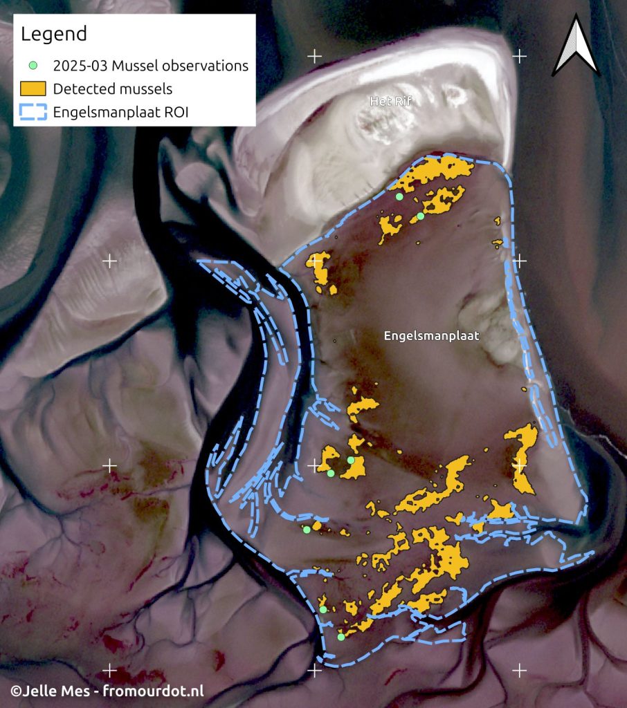
Fig. 8 shows a map of detected mussels on 2025-03-01 within the ROI. There are several large mussel reefs visible which match the field observations. There are some false detections on the northeast side, but they are rather small and will not have a large impact on the overall surface statistics derived later on. Dark patches on the mudflat extend beyond the orange polygons, suggesting that the mussel reefs are larger than currently detected. This could be due to the reefs not protruding above the still standing water on the mudflats or the mussels not being large enough to cause significant backscatter. These dark patches could also be algae as nearly all of them have high NDVI values, indicating a high chlorophyll content.
Batch processing the 24 monthly VH images gives 24 vector layers, visualized as an animation in Fig. 9. An explosive growth in detected mussels can be seen in August 2024. Just before there are two images which seem to contain many false detections. These are from 2024-05-12 and 2024-07-09. It might be possible that clumps of larger mussels show up these months randomly dispersed over the shoal before being washed away and only the more consolidated reefs continue their growth.
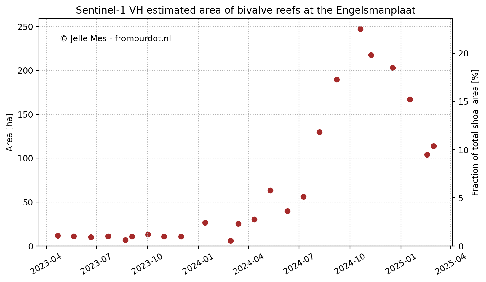
The total area of these polygons per month is plotted in Fig. 10, showing a large peak in the second half of 2024. In 2023 the area of the reefs is rather stable, between 6.8 and 13.2 hectares, or 0.6 and 1.2% of the total area of the Engelsmanplaat. At the start of 2024 the area grows to 30 hectares and then jumps up in the late summer months, peaking at 247 hectares on 2024-10-20, 22.5% of the mudflat area. During the subsequent winter it falls back down to around 110 hectares, 10% of the mudflat.
Discussion & Conclusion
The estimated reef area at the start of 2023 is a bit lower than that reported by WMR, shown in Fig. 2: ~14 hectares. These measurements do not take gaps in the middle of the reefs into account, the polygons are outlines of the reefs only. This explains the lower reef area from the SAR method presented here. The start of the explosive growth in Fig. 10 around July 2024 coincides with the first sightings from the volunteers of Staatsbosbeheer , see also Fig. 3 and 4. It is suspected that at this stage the mussels became large enough to be picked up by the C-band radar, being around 6 to 10 mm in size. This aligns with the primary length-wise growth period for mussels between april and august . Around half of the new mussel reefs do not survive the winter of 2025, matching winter survival rates from the literature, usually around 60% .
The distribution of detected mussel reefs align with field observations and the general pattern that the volunteers of Staatsbosbeheer observe in the area. Especially the reefs at the northern edge of the Engelsmanplaat can be reliably mapped to known mussel reefs due to frequent visits by the volunteers. The aforementioned noise in 2024-05 and 2024-07 is an issue, but could be partially filtered out using one of the digital elevation models (DEMs) of the region that are available (e.g. Kustlidar, JarKus, vaklodingen or AHN) using the previously mentioned long term survival threshold of +0.1 m NAP. Note that the new, south-eastern mussel reef on the north side of the Engelsmanplaat is located between +0.05 and +0.20 m NAP, right at this threshold. Filtering above +0.40 m NAP would suffice in this case. Temporal stacking of SAR images would also reduce speckle noise, at the cost of temporal resolution. With the start of Sentinel-1C operations in April 2025 the higher imaging cadence could support such a strategy while still enabling reef mapping on a month basis.
To my knowledge, this is the first case of the growth of mussel reefs being tracked on such a high cadence in a relatively large area. It provides detailed insight into the development of individual reefs and the population as a whole. With two Sentinel-1 satellites operational at the end of 2025 and one additional having been launched, the availability of imagery will increase dramatically. This will enable mapping the effects of individual storms on the conditions of the reefs. Further opportunities arise by increasing the area of the Wadden Sea being monitored with this technique. It can be easily scaled up to the entire Dutch Wadden Sea, as long as vegetated (land) areas are avoided. This would entail an increase in surveyed area from 11 to 2296 km^2, excluding the Dollard. Historical Sentinel-1 data going back to 2016 can be used to quickly obtain a mussel reef development timeline that can be compared to existing methods.
Regarding the development of the mussel reefs themselves, a large unknown is whether the new reefs will be stable in the coming years. Survival rates are generally poor: around 50% after the first winter and dropping to 20% after 6 winters compared to the first year . However, even with a 20% survival rate, the peak of ~200 ha in October-December 2024 would be reduced to ~40 ha over 6 years, a 4 fold increase in area compared to 2023.